Note
Click here to download the full example code
LineageOT on a curled trajectory
This shows results of applying LineageOT to a simulation where descendant cells are not all closest to their ancestors, closely following simulation_demo.ipynb in the source code.
import copy
import matplotlib.pyplot as plt
import numpy as np
import ot

import lineageot.simulation as sim
import lineageot.evaluation as sim_eval
import lineageot.inference as sim_inf
Generating simulated data
flow_type = 'mismatched_clusters'
np.random.seed(257)
Setting simulation parameters
if flow_type == 'bifurcation':
    timescale = 1
else:
    timescale = 100

x0_speed = 1/timescale


sim_params = sim.SimulationParameters(division_time_std = 0.01*timescale,
                                      flow_type = flow_type,
                                      x0_speed = x0_speed,
                                      mutation_rate = 1/timescale,
                                      mean_division_time = 1.1*timescale,
                                      timestep = 0.001*timescale
                                     )

mean_x0_early = 2
time_early = 4*timescale # Time when early cells are sampled
time_late = time_early + 4*timescale # Time when late cells are sampled
x0_initial = mean_x0_early -time_early*x0_speed
initial_cell = sim.Cell(np.array([x0_initial, 0, 0]), np.zeros(sim_params.barcode_length))
sample_times = {'early' : time_early, 'late' : time_late}

# Choosing which of the three dimensions to show in later plots
if flow_type == 'mismatched_clusters':
    dimensions_to_plot = [1,2]
else:
    dimensions_to_plot = [0,1]
Running the simulation
sample = sim.sample_descendants(initial_cell.deepcopy(), time_late, sim_params)
Processing simulation output
# Extracting trees and barcode matrices
true_trees = {'late':sim_inf.list_tree_to_digraph(sample)}
true_trees['late'].nodes['root']['cell'] = initial_cell
true_trees['early'] = sim_inf.truncate_tree(true_trees['late'], sample_times['early'], sim_params)
# Computing the ground-truth coupling
couplings = {'true': sim_inf.get_true_coupling(true_trees['early'], true_trees['late'])}
data_arrays = {'late' : sim_inf.extract_data_arrays(true_trees['late'])}
rna_arrays = {'late': data_arrays['late'][0]}
barcode_arrays = {'late': data_arrays['late'][1]}
rna_arrays['early'] = sim_inf.extract_data_arrays(true_trees['early'])[0]
num_cells = {'early': rna_arrays['early'].shape[0], 'late': rna_arrays['late'].shape[0]}
print("Times : ", sample_times)
print("Number of cells: ", num_cells)
# Creating a copy of the true tree for use in LineageOT
true_trees['late, annotated'] = copy.deepcopy(true_trees['late'])
sim_inf.add_node_times_from_division_times(true_trees['late, annotated'])
sim_inf.add_nodes_at_time(true_trees['late, annotated'], sample_times['early']);
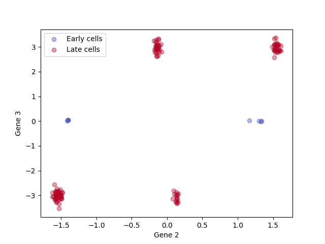
# Scatter plot of cell states
cmap = "coolwarm"
colors = [plt.get_cmap(cmap)(0), plt.get_cmap(cmap)(256)]
for a,label, c in zip([rna_arrays['early'], rna_arrays['late']], ['Early cells', 'Late cells'], colors):
plt.scatter(a[:, dimensions_to_plot[0]], a[:, dimensions_to_plot[1]], alpha = 0.4, label = label, color = c)
plt.xlabel('Gene ' + str(dimensions_to_plot[0] + 1))
plt.ylabel('Gene ' + str(dimensions_to_plot[1] + 1))
plt.legend();
Out:
Times    :  {'early': 400, 'late': 800}
Number of cells:  {'early': 8, 'late': 128}

<matplotlib.legend.Legend object at 0x7f69ee2be3d0>
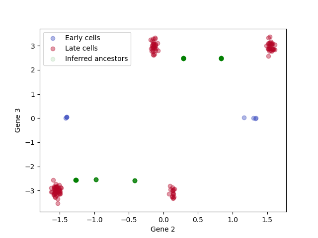
Since these are simulations, we can compute and plot inferred ancestor locations based on the true tree.
# Infer ancestor locations for the late cells based on the true lineage tree
observed_nodes = [n for n in sim_inf.get_leaves(true_trees['late, annotated'], include_root=False)]
sim_inf.add_conditional_means_and_variances(true_trees['late, annotated'], observed_nodes)

ancestor_info = {'true tree':sim_inf.get_ancestor_data(true_trees['late, annotated'], sample_times['early'])}

# Scatter plot of cell states, with inferred ancestor locations for the late cells

for a,label, c in zip([rna_arrays['early'], rna_arrays['late']], ['Early cells', 'Late cells'], colors):
    plt.scatter(a[:, dimensions_to_plot[0]], a[:, dimensions_to_plot[1]], alpha = 0.4, label = label, color = c)

plt.scatter(ancestor_info['true tree'][0][:,dimensions_to_plot[0]],
            ancestor_info['true tree'][0][:,dimensions_to_plot[1]],
            alpha = 0.1,
            label = 'Inferred ancestors',
            color = 'green')
plt.xlabel('Gene ' + str(dimensions_to_plot[0] + 1))
plt.ylabel('Gene ' + str(dimensions_to_plot[1] + 1))
plt.legend();
Out:
<matplotlib.legend.Legend object at 0x7f69e618fed0>
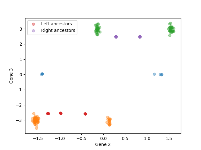
To better visualize cases where there were two clusters at the early time point, we can color the late cells (and their inferred ancestors) by their cluster of origin Cells in orange are from the late time point with ancestors on the left; cells in green are from the late time point with ancestors on the right. The estimated ancestor distributions in red and purple are closer to the true ancestors than the observations in orange and green.
is_from_left = sim_inf.extract_ancestor_data_arrays(true_trees['late'], sample_times['early'], sim_params)[0][:,1] < 0
for a,label in zip([rna_arrays['early'], rna_arrays['late'][is_from_left,:], rna_arrays['late'][~is_from_left,:]], ['Early cells', 'Late cells from left', 'Late cells from right']):
    plt.scatter(a[:, 1], a[:, 2], alpha = 0.4)

plt.xlabel('Gene 2')
plt.ylabel('Gene 3')


for a, label in zip([ancestor_info['true tree'][0][is_from_left, :], ancestor_info['true tree'][0][~is_from_left, :]], ['Left ancestors', 'Right ancestors']):
    plt.scatter(a[:,1], a[:,2], alpha = 0.4, label = label)
plt.legend()
Out:
<matplotlib.legend.Legend object at 0x7f69ee2eb910>
Running LineageOT
The first step is to fit a lineage tree to observed barcodes
# True distances
true_distances = {key:sim_inf.compute_tree_distances(true_trees[key]) for key in true_trees}


# Estimate mutation rate from fraction of unmutated barcodes
rate_estimate = sim_inf.rate_estimator(barcode_arrays['late'], sample_times['late'])

# Compute Hamming distance matrices for neighbor joining
hamming_distances_with_roots = {'late':sim_inf.barcode_distances(np.concatenate([barcode_arrays['late'],
                                                                                 np.zeros([1,sim_params.barcode_length])]))}

# Compute neighbor-joining tree
fitted_tree = sim_inf.neighbor_join(hamming_distances_with_roots['late'])
Once the tree is computed, we need to annotate it with node times and states
# Annotate fitted tree with internal node times
sim_inf.add_leaf_barcodes(fitted_tree, barcode_arrays['late'])
sim_inf.add_leaf_x(fitted_tree, rna_arrays['late'])
sim_inf.add_leaf_times(fitted_tree, sample_times['late'])
sim_inf.annotate_tree(fitted_tree,
                  rate_estimate*np.ones(sim_params.barcode_length),
                  time_inference_method = 'least_squares');

# Add inferred ancestor nodes and states
sim_inf.add_node_times_from_division_times(fitted_tree)
sim_inf.add_nodes_at_time(fitted_tree, sample_times['early'])
observed_nodes = [n for n in sim_inf.get_leaves(fitted_tree, include_root = False)]
sim_inf.add_conditional_means_and_variances(fitted_tree, observed_nodes)
ancestor_info['fitted tree'] = sim_inf.get_ancestor_data(fitted_tree, sample_times['early'])
Out:
     pcost       dcost       gap    pres   dres
 0: -4.0661e+07 -4.2066e+07  6e+06  1e-01  2e-01
 1: -4.0696e+07 -4.1441e+07  8e+05  8e-03  2e-02
 2: -4.0803e+07 -4.1023e+07  2e+05  2e-03  4e-03
 3: -4.0851e+07 -4.0887e+07  4e+04  1e-16  1e-16
 4: -4.0862e+07 -4.0866e+07  4e+03  1e-16  2e-16
 5: -4.0863e+07 -4.0864e+07  3e+02  1e-16  2e-16
 6: -4.0863e+07 -4.0863e+07  1e+01  1e-16  4e-16
Optimal solution found.
We’re now ready to compute LineageOT cost matrices
# Compute cost matrices for each method
coupling_costs = {}
coupling_costs['lineageOT, true tree'] = ot.utils.dist(rna_arrays['early'], ancestor_info['true tree'][0])@np.diag(ancestor_info['true tree'][1]**(-1))
coupling_costs['OT'] = ot.utils.dist(rna_arrays['early'], rna_arrays['late'])
coupling_costs['lineageOT, fitted tree'] = ot.utils.dist(rna_arrays['early'], ancestor_info['fitted tree'][0])@np.diag(ancestor_info['fitted tree'][1]**(-1))


early_time_rna_cost = ot.utils.dist(rna_arrays['early'], sim_inf.extract_ancestor_data_arrays(true_trees['late'], sample_times['early'], sim_params)[0])
late_time_rna_cost = ot.utils.dist(rna_arrays['late'], rna_arrays['late'])
Given the cost matrices, we can fit couplings with a range of entropy parameters.
epsilons = np.logspace(-2, 3, 15)

couplings['OT'] = ot.emd([],[],coupling_costs['OT'])
couplings['lineageOT'] = ot.emd([], [], coupling_costs['lineageOT, true tree'])
couplings['lineageOT, fitted'] = ot.emd([], [], coupling_costs['lineageOT, fitted tree'])
for e in epsilons:
    if e >=0.1:
        f = ot.sinkhorn
    else:
        # Epsilon scaling is more robust at smaller epsilon, but slower than simple sinkhorn
        f = ot.bregman.sinkhorn_epsilon_scaling
    couplings['entropic rna ' + str(e)] = f([],[],coupling_costs['OT'], e)
    couplings['lineage entropic rna ' + str(e)] = f([], [], coupling_costs['lineageOT, true tree'], e*np.mean(ancestor_info['true tree'][1]**(-1)))
    couplings['fitted lineage rna ' + str(e)] = f([], [], coupling_costs['lineageOT, fitted tree'], e*np.mean(ancestor_info['fitted tree'][1]**(-1)))
Out:
/home/docs/checkouts/readthedocs.org/user_builds/lineageot/envs/latest/lib/python3.7/site-packages/ot/bregman.py:1112: UserWarning: Sinkhorn did not converge. You might want to increase the number of iterations `numItermax` or the regularization parameter `reg`.
  warnings.warn("Sinkhorn did not converge. You might want to "
/home/docs/checkouts/readthedocs.org/user_builds/lineageot/envs/latest/lib/python3.7/site-packages/ot/bregman.py:517: UserWarning: Sinkhorn did not converge. You might want to increase the number of iterations `numItermax` or the regularization parameter `reg`.
  warnings.warn("Sinkhorn did not converge. You might want to "
Evaluation of couplings
First compute the independent coupling as a reference
couplings['independent'] = np.ones(couplings['OT'].shape)/couplings['OT'].size
ind_ancestor_error = sim_inf.OT_cost(couplings['independent'], early_time_rna_cost)
ind_descendant_error = sim_inf.OT_cost(sim_eval.expand_coupling(couplings['independent'],
                                                                couplings['true'],
                                                                late_time_rna_cost),
                                       late_time_rna_cost)
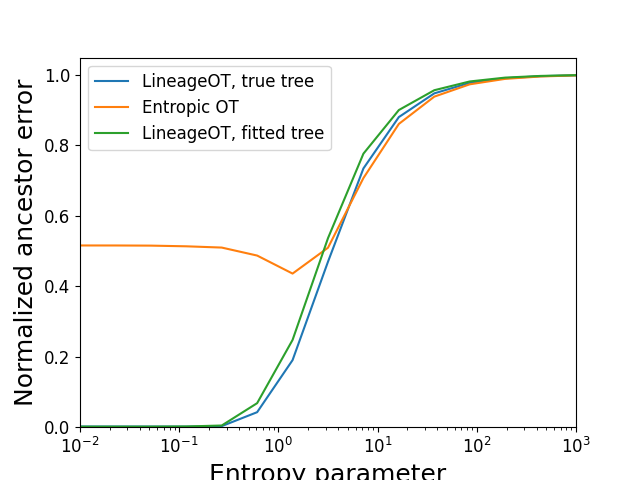
Plotting the accuracy of ancestor prediction
ancestor_errors = sim_eval.plot_metrics(couplings,
                                        lambda x:sim_inf.OT_cost(x, early_time_rna_cost),
                                        'Normalized ancestor error',
                                        epsilons,
                                        scale = ind_ancestor_error,
                                        points=False)
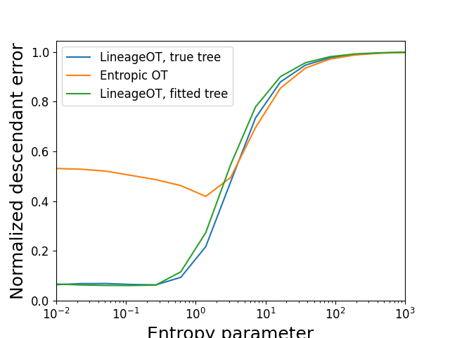
Plotting the accuracy of descendant prediction
descendant_errors = sim_eval.plot_metrics(couplings,
                                          lambda x:sim_inf.OT_cost(sim_eval.expand_coupling(x,
                                                                                            couplings['true'],
                                                                                            late_time_rna_cost),
                                                                   late_time_rna_cost),
                                          'Normalized descendant error',
                                          epsilons, scale = ind_descendant_error)
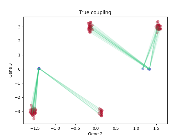
Coupling visualizations
Visualizing the ground-truth coupling, zero-entropy LineageOT coupling, and zero-entropy optimal transport coupling.
Ground truth:
sim_eval.plot2D_samples_mat(rna_arrays['early'][:, [dimensions_to_plot[0],dimensions_to_plot[1]]],
                   rna_arrays['late'][:, [dimensions_to_plot[0],dimensions_to_plot[1]]],
                   couplings['true'],
                   c=[0.2, 0.8, 0.5],
                   alpha_scale = 0.1)

plt.xlabel('Gene ' + str(dimensions_to_plot[0] + 1))
plt.ylabel('Gene ' + str(dimensions_to_plot[1] + 1))
plt.title('True coupling')


for a,label, c in zip([rna_arrays['early'], rna_arrays['late']], ['Early cells', 'Late cells'], colors):
    plt.scatter(a[:, dimensions_to_plot[0]], a[:, dimensions_to_plot[1]], alpha = 0.4, label = label, color = c)
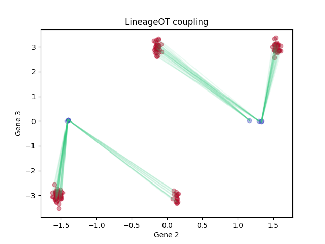
LineageOT:
sim_eval.plot2D_samples_mat(rna_arrays['early'][:, [dimensions_to_plot[0],dimensions_to_plot[1]]],
                   rna_arrays['late'][:, [dimensions_to_plot[0],dimensions_to_plot[1]]],
                   couplings['lineageOT'],
                   c=[0.2, 0.8, 0.5],
                   alpha_scale = 0.1)
plt.xlabel('Gene ' + str(dimensions_to_plot[0] + 1))
plt.ylabel('Gene ' + str(dimensions_to_plot[1] + 1))
plt.title('LineageOT coupling')

for a,label, c in zip([rna_arrays['early'], rna_arrays['late']], ['Early cells', 'Late cells'], colors):
    plt.scatter(a[:, dimensions_to_plot[0]], a[:, dimensions_to_plot[1]], alpha = 0.4, label = label, color = c)
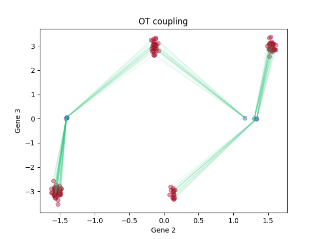
Optimal transport
sim_eval.plot2D_samples_mat(rna_arrays['early'][:, [dimensions_to_plot[0],dimensions_to_plot[1]]],
                   rna_arrays['late'][:, [dimensions_to_plot[0],dimensions_to_plot[1]]],
                   couplings['OT'],
                   c=[0.2, 0.8, 0.5],
                   alpha_scale = 0.1)
plt.xlabel('Gene ' + str(dimensions_to_plot[0] + 1))
plt.ylabel('Gene ' + str(dimensions_to_plot[1] + 1))
plt.title('OT coupling')


for a,label, c in zip([rna_arrays['early'], rna_arrays['late']], ['Early cells', 'Late cells'], colors):
    plt.scatter(a[:, dimensions_to_plot[0]], a[:, dimensions_to_plot[1]], alpha = 0.4, label = label, color = c)
Total running time of the script: ( 0 minutes 9.832 seconds)